Our last post (article III) covered radio frequency spectrum bands and their applications. However, the primary reason for starting this series is to develop both theoretical and practical knowledge of DSP. Over time, readers can expect an Applied DSP series to be published concurrently. In this article, we will focus on topics covered in Chapter One of Lyons’s Understanding Digital Signal Processing (UDSP) (specifically Discrete Sequences and Systems). The intuition behind the distinction between discrete and continuous waveforms should become unquestionably clear after this post. Furthermore, we will demonstrate the benefits of representing physical measurements in either form. The notation associated with each will be discussed, and we will use Python’s Matplotlib library to graphically illustrate their key differences. In addition, we will carefully evaluate the contrast between signal amplitude, magnitude, and power. Finally, basic signal processing operations will be introduced, and we will use Draw.io to construct DSP block diagrams.

Discrete Sequences and Continuous Waveforms

From our intuition, one might think that the characterization of a discrete sequence from a continuous waveform is fully distinct. Mathematically, they are quite different; however, in engineering, we must often accept that physical hardware has limits, and thus, it is sometimes appropriate to treat certain sequences as continuous for analysis purposes. For example, satellite monitoring of space weather requires many sensors that periodically sample measurements, relaying this information to nearby ground stations. Disregarding the fundamental principles of modern physics that may dictate the granularity of nature, conceptually, these sensors are mapping continuous physical phenomena into discrete sequences of measurements taken at discrete time intervals ().

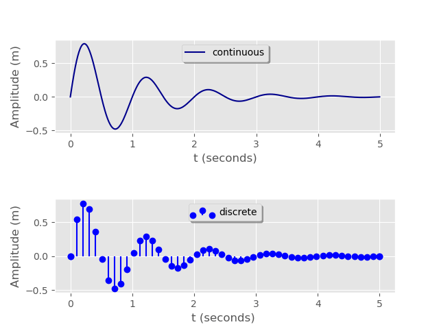
For now we will concern ourselves only with signals whose time domain is quantized; we will focus on signals with discretized amplitudes in later articles. The difference between continuous waveforms and discrete sequences is depicted in the graphic below:

import matplotlib
import matplotlib.pyplot as plt
import numpy as np

num_samples = 50
t_1 = np.arange(0.0, 5.0, 0.01)
t_2 = np.linspace(0.0, 5.0, num_samples)

def damped_sin(t):
     return np.exp(-t)*np.sin(2*np.pi*t)

matplotlib.style.use('ggplot')
plt.figure(1)
plt.subplot(211)
plt.plot(t_1, damped_sin(t_1), label = 'continuous', color = 'darkblue')
plt.xlabel('t (seconds)')
plt.ylabel('Amplitude (m)')
legend = plt.legend(loc='upper center', shadow=True)

plt.subplot(212)
plt.stem(t_2, damped_sin(t_2), label = 'discrete', markerfmt='bo', linefmt = 'bo', basefmt = 'bo')
plt.xlabel('t (seconds) ')
plt.ylabel('Amplitude (m)')
legend = plt.legend(loc='upper center', shadow=True)
plt.subplots_adjust(hspace=0.7)
# plt.savefig("damped_sin.png")
plt.show()

Lyons used the sinusoidal function as his example to illustrate the distinction, but the upper graph depicts a common scenario known as the damped sinusoidal wave. The continuous and discrete equations are presented, respectively:

Continuous Waveform

Discrete Sequence

where is the absolute frequency of the signal, is zero or any positive integer, and is the sample period, i.e. the amount of time per sample. Therefore, we can compute the sample frequency of as . From the discrete graph above, we observe that each plot extends up to 5 seconds, and our code indicates that 50 samples were taken in this timeframe. Therefore we can compute:

and the sample frequency would then be 10 samples per second. The point of this, however, is to highlight the rich connection between and . In fact, if we know the number of samples per oscillation — which, from the graph, appears to be 10 samples per oscillation — we can use to find the period of the wave itself:

… and we understand, from article III, the inverse relationship between the period of and its frequency: . Over time, we will learn more about the relationship between and . For now we will look more into the distinction between signal amplitude, magnitude, and power.

Signal Amplitude, Magnitude, and Power

It’s interesting to see why Mr. Lyons readily made a distinction between these concepts. Spending so many years as the lead hardware engineer at the National Security Agency and Northrop Grumman Corp, he likely encountered many people who mistakenly used them interchangeably. This section may be summarized with the following chart:

Name	Notation	Description
Signal Amplitude		A raw, unsigned, instantaneous sample value.
Magnitude		The absolute value of the signal amplitude (always non-negative).
Power		The squared magnitude; represents the power of the sample.

DSP Block Diagrams

Now we will talk a little bit about some of the common graphical operational symbols used for signal processing, and how they might be used to demonstrate complex systems. One can more broadly see these operations as a transformation of some input digital signal to a digital output, which will be called a “system”. The Draw.io software would be really helpful to us in the future, for constructing these systems. Our most fundamental, addition, subtraction, summation, multiplication, and Unit delay are demonstrated below:

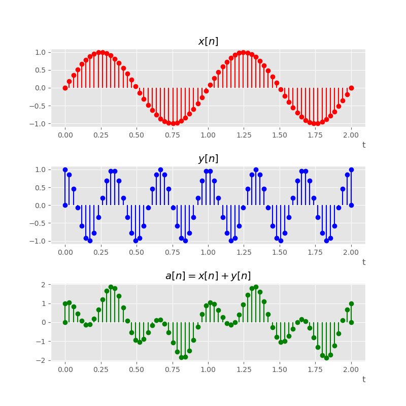
Addition

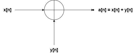
The addition operator is represented by a circle and a cross. As we can see from the graphic above, it takes the inputs and and returns the output . This can be interpreted as the addition of two discrete signals, as depicted in the image below:

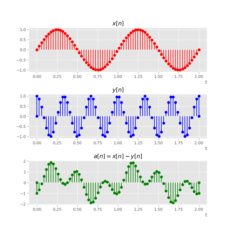
Subtraction

Subtraction can be viewed as addition where the input signal is first inverted. That is, subtracting is equivalent to adding . An example of this operation is shown below, where sine waves of two distinct frequencies are subtracted for the resulting waveform :

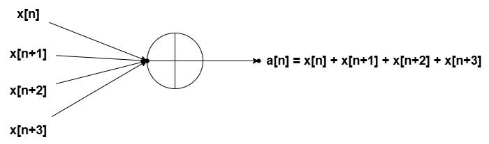
Summation

Another common operation useful in DSP is the summation operator. This operator iteratively takes a specified number of consecutive values as inputs and produces their sum as the output. The number of values taken as input is called the window of the summation. For example, the window in the diagram below equals 3.

Let’s take a look at the table below:

Here we see that the input is . The columns to the right show the outputs after applying summation operators with window sizes of 2 and 3, respectively.

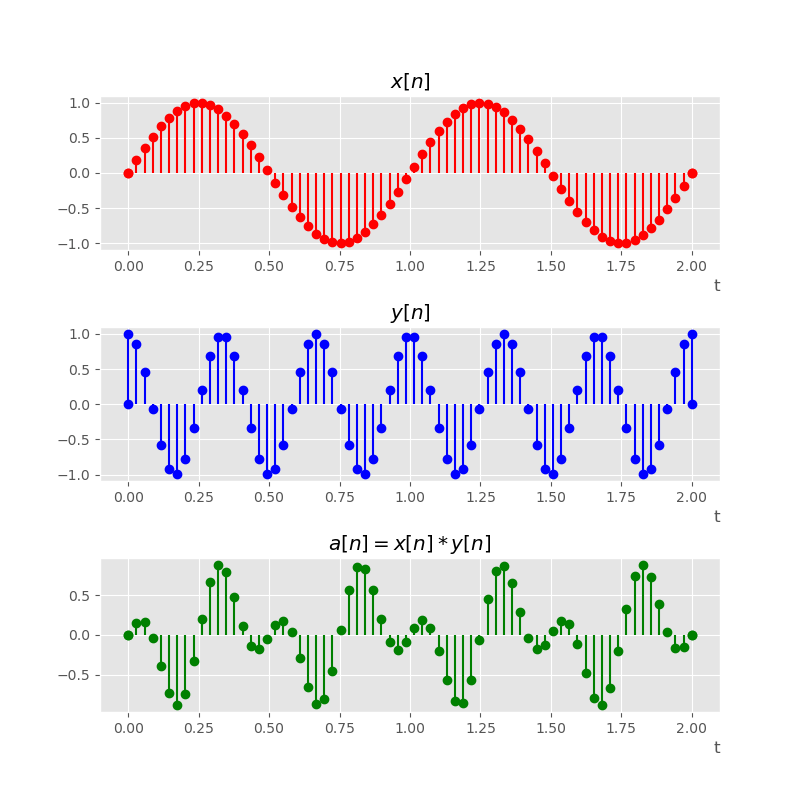
Multiplication

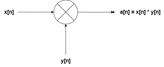
Multiplying waveforms is pretty straightforward. Similar to addition and subtraction, it requires two input sequences, but it returns the product of those sequences.

Unit Delay

Finally, we have the unit delay, the fundamental building block that shifts an input sequence by one sample. It implements the mapping

for all . The diagram below shows its standard representation:

The table that follows summarizes how each input value is shifted. At , since is undefined, the output is typically initialized to zero (or marked “NaN” to mean “not a number” in some computational systems). Let’s examine the table:

Having distinguished discrete from continuous waveforms, reviewed key signal metrics, and explored foundational block diagrams, we’re now ready to dive into Part II (an in-depth study of linear and nonlinear systems and their practical applications).