So far we have established several mathematical cornerstones of DSP. Particularly in articles I and II, we covered complex numbers, the closed-form of geometric series, logarithms, and metric prefixes. Now we’ll turn our attention to another foundational pillar of this study: developing an intuition for frequency, as well as understanding the Radio Frequency Spectrum bands and their applications.

What is Frequency Anyway?

So we talked a little bit about the angular frequency of a waveform in article I, but we did not yet clarify what it fully means dimensionally. One of the most effective tools for gaining intuition about concepts in physics and engineering, is a subfield called dimensional analysis (or the factor-label method). This entails writing out a physics equation in its most general form using our most fundamental dimension symbols: [T] for time, [L] for length, [M] for mass and so on. For example, we know the speed of an object is measured by dividing the distance traveled by the amount of time that it took to travel that length… or more concisely we have the dimensional equation:

The wavelength of a signal is measured in units of length, and would merely be represented by . Previously we stated that frequency is measured in Hertz, or cycles per second. Moreover we learned that cycle itself is a dimensionless quantity, leading us to represent the dimension of frequency like so:

This form allows us to further understand the relationship between frequency and other related measures. For example, it is a well known physical property in the mechanics of a wave, that we can express the frequency of a wave traversing in a medium with the following equation:

where is the speed of the wave traveling in that medium, and is the signal’s wavelength. Dimensionally this makes sense, as we can now substitute the dimensional forms of speed and wavelength in this equation to simplify frequency back to its basic form:

Frequency is often concretely represented as the ratio , where denotes the time required for one complete cycle of the waveform. This is known as the period of the signal. Frequency is a fundamental property of nature, and a deep understanding of its various aspects is essential for mastering its applications. In the following section, we will examine the RF spectrum bands and their uses in greater detail.

Radio Frequency Spectrum Bands

Signal frequencies lie in a mathematical continuum, collectively known as the spectrum. Engineers and scientists, recognizing distinct physical and functional characteristics in these ranges, have subdivided them into different bands. Though Richard Lyons’s text does not explore this topic explicitly, I believe a clear understanding of the RF spectrum and its practical subdivisions is critical to any serious exploration of DSP.

To begin with, our focus within the RF spectrum will be limited to the higher range of metric prefixes. Specifically, we’ll dissect those introduced under The Great Monkey King mnemonic in article II (and reiterated in the table below):

“The”	“Great”	“Monkey”	“King”
Tera –	Giga –	Mega –	Kilo –
T	G	M	K

The motto of BGecko, prominently shown on the homepage, displays a timeless insight from Leonardo da Vinci: “Learn how to See.” Although the visible spectrum is in the vicinity of 400 – 760 THz, learning to see also entails recognizing those frequencies of light that lie beyond the reach of the naked eye. To better understand these invisible frequencies, we propose the mnemonic VUSE, an intentional eye dialect of “views”, standing for “Very-“, “Ultra-“, “Super-” and “Extremely-” prefixes. The table below shows how VUSE can be used to help order the frequencies:

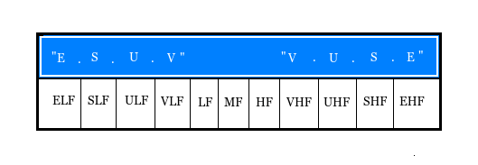
Observe that at the center of the table lie LF, MF, and HF, denoting Low, Medium, and High Frequencies respectively. As we move outward from the middle both LF and HF are expanded using the VUSE prefixes, respectively reflecting decreasing and increasing orders of magnitude. The table below further characterizes how these orders of magnitudes are split in the spectrum:

ELF	3 – 30 Hz
SLF	30 – 300 Hz
ULF	300 Hz – 3 kHz
VLF	3 – 30 kHz
LF	30 – 300 kHz
MF	300 KHz – 3 MHz
HF	3 – 30 MHz
VHF	30 – 300 MHz
UHF	300 MHz – 3 GHz
SHF	3 – 30 GHz
EHF	30 – 300 GHz

The ELF band begins at 3 Hz and extends up to 30 Hz, spanning a single order of magnitude. The SLF band picks up precisely at 30 Hz and extends to 300 Hz, again covering one full order. This progression systematically continues up the spectrum, culminating in the EHF band, which ranges from 30 GHz to 300 GHz.

NTIA’s US Frequency Allocations Table

Now that we classified the RF range from 3 Hz to 300 GHz, this allows us to assign specific applications within the spectrum. The National Telecommunications and Information Administration provides an accessible diagram detailing band usage, shown below: