Advanced –A Treatise on Parametric Forms of Multimodal Distributions

This document is part of a developing theoretical framework authored by Christopher Lee Burgess.

Abstract

Classical variance is insufficient for characterizing the geometric structure of multimodal data. In this work, we will define a new quantity called the pseudovariance, and demonstrate how it captures shape, modality, and dispersion through a general class of functions we call “forma”. By contrasting this novel interpretation of variance with classical variance, we reveal how non-localized behavior forces us to tweak the traditional axiomatic framework. From this, we will provide a closed analytic form for multimodal distributions and demonstrate how it corresponds with other members of the exponential family. Finally, we will explore the rich connections between pseudovariance and unimodal moment behavior.

Key Words: Pseudovariance, Multimodal, Variance, Analytic Form.

Introduction

It is sort of ironic, that there has been significant variation in our formulation of variance in many chapters of statistical lineage. For now, we will focus on the one-dimensional case. If we define the mapping $\phi(x) = (x - \mu)^{2}$ for variable $x$ and parameter $\mu$ in $\mathbb{R}$ , this classical variance can be described with the following formula:

$\displaystyle \text{VAR}(X) = \mathbb{E}[\phi(X)]$

where the parameter $\mu = \mathbb{E}[X]$ is the mean of our data. The graphic below illustrates $\phi$ ‘s contribution to our classical measure:

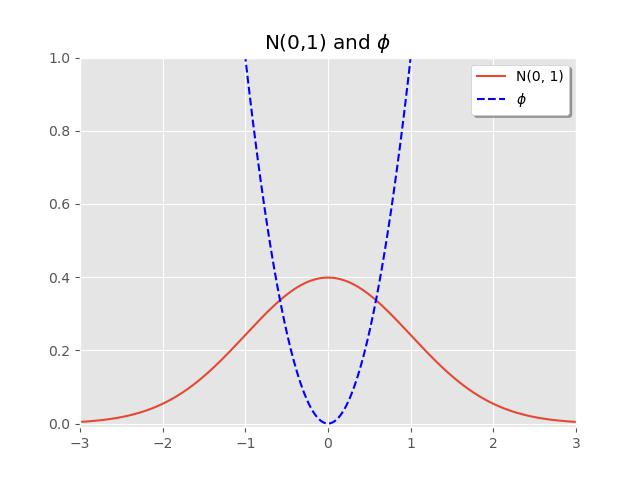
From this, we can interpret that the farther out a sampled data point $x_{*}$ is from the mean, which is zero in this case, there is a higher contribution $\phi(x_{*})$ to our variance quantity measure.

Historically classical variance has been shown to satisfy a certain set of preliminary axioms and assumptions, enumerated below:

Axiom 0

If our random variable $X = c$ , for some constant $c \in \mathbb{R}$ , then $\text{VAR}(X) = 0$ .

Axiom 1

(Positivity)

If $X \neq c$ , then $\text{VAR}(X) > 0$ .

Assumption 0

(Localization Invariance)
For any constant $c$ , we have the property $\text{VAR}(X+c) = \text{VAR}(X)$ .

Assumption 1

For any constant $c$ , we have the property $\text{VAR}(cX) = c^{2}\text{VAR}(X)$ .

However, one key point of this article, is that classical variance inherently assumes a unimodal central tendency and does not fully characterize the spread for multimodal distributions. To provide an example, we define the distribution $\mathcal{D} = 0.5 N(-3, 1) + 0.5 N(3, 1)$ . If we continually sample from $\mathcal{D}$ , the equal weighting of Gaussians $N(-3, 1)$ and $N(3, 1)$ would grant us a sample mean that converges to zero, but clearly $\phi$ doesn’t adequately capture the concentration of data around the modes:

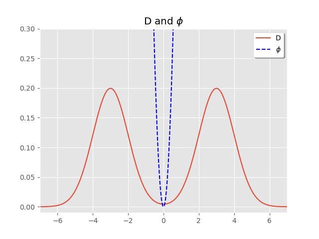
On first glance, given the shape of this bimodal distribution, we can guess that $\phi(x) = k (x^{2} - 9)^{2}$ , for some positive constant $k$ . From this we observe more robust contributions to dispersion for $\mathcal{D}$ :

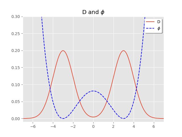
We can see how, by letting $\phi$ be of this form, our pseudo variance violates the localization assumption above. Later in our research, we will find that this not a bug, but a feature of this generalization. However, it is important to first formalize our definitions in order to gain a richer understanding about what is being conveyed here.

On Pseudovariance

To formalize these concepts related to pseudovariance and multimodal distributions, I’ll first introduce a few definitions:

Definition 1 (Pseudovariance) Given some distribution $\mathcal{D}$ over random variable $X$ and positive semidefinite function $\phi: X \longrightarrow \mathbb{R} \cup \{ \infty\}$ , the corresponding pseudovariance is as follows:

$\displaystyle \Sigma_{\phi} = \text{VAR}_{\phi}(X) = \mathbb{E}[\phi(X)]$

And we will refer to $\phi$ as the forma function, since “forma” is latin for “shape”. Later we will see it is important to choose forma $\phi$ , such that $\Sigma_{\phi}$ satisfies axioms 0 and 1 from our classical variance. Essentially this definition relaxes the assumptions stated above.

Definition 2 (Pseudocovariance) Let $\mathcal{D}$ be a probability distribution over the random variable $S = X \times Y$ , and let $\phi : S \longrightarrow \mathbb{R} \cup \{\infty\}$ be a positive semidefinite, measurable function. Then the pseudocovariance of $X$ and $Y$ with respect to $\phi$ is define as:

$\displaystyle \text{COV}_{\phi}(X, Y) = \mathbb{E}[\phi(X,Y)]$

Definition 3 (Local Minimum) For any smooth function $\phi(x)$ , we say the point $x_{\star}$ achieves a local minimum $\phi(x_{\star})$ if and only if $\phi'(x_{\star}) = 0$ and $\phi''(x_{\star}) > 0$ .

Definition 4 (Pseudomean) Given any pseudovariance $\Sigma_{\phi}$ over $\mathcal{D}$ , define the set $M = \{ x \in X | \phi(x) \text{ is a local minimum}\}$ , and every $\mu \in M$ will be called a pseudomean of $\mathcal{D}$ .

So for example,

In the standard unimodal case, we let $\phi(x) = (x - \mu)^{2}$ , and thus $M = \{\mu \}$ .

Or in the standard bimodal case, where if we let $\phi(x) = k(x^{2} - \beta)^{2}$ , we can show $M = \{-\sqrt{\beta}, \sqrt{\beta} \}$ .

In this treatise, we might later consider those critical points of the forma function which are not local minima, but for now let’s move into moments.

For any positive integer $k$ , let $\phi^{-k}(x)$ be the $k^{th}$ order antiderivative with all constants of integration equal to zero. Then the definition of the $k^{th}$ order moment under this framework is as follows:

Definition 5. (Moments) Let $\mathcal{D}$ be any distribution over the random variable $X$ , and $\phi$ be our forma function. Then the $k^{th}$ order moment is given by the equation

$\displaystyle \mu_{k} := \frac{k!}{2}\mathbb{E}[\phi^{(2-k)}(X)]$

So in the classical framework, by letting our forma function be $\phi(x) = (x - \mu)^{2}$ , we know that $\phi^{-1}(x) = \frac{1}{3}(x - \mu)^{3}$ . Therefore, our third order moment can be expressed like so:

$\displaystyle \mu_{3} = \frac{3!}{2}\mathbb{E}[\phi^{-1}(X)] = \frac{3!}{2}\mathbb{E}[\frac{1}{3}(X - \mu)^{3}]$

$\displaystyle = \mathbb{E}[(X - \mu)^{3}]$

which aligns with the classical interpretation of the $3^{rd}$ order moment. Throughout this treatise, the quantity $\varepsilon_{k}$ will be used to explicitly refer to the $k^{th}$ order classical moment.

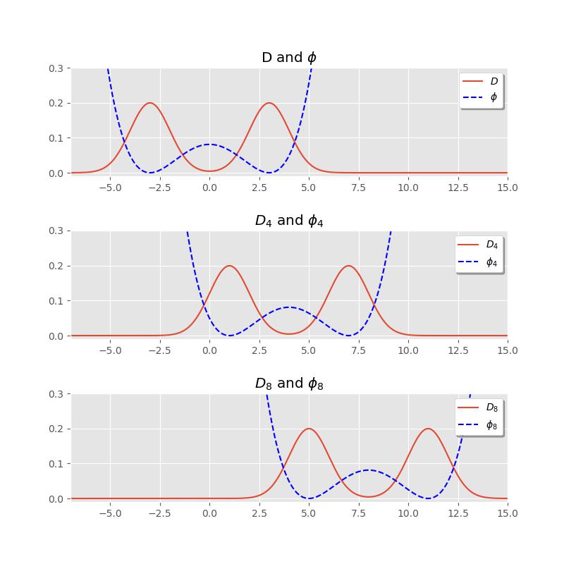
Definition 6 (Center translation of forma) Let $\mathcal{D}$ be a distribution over the random variable $X$ , and let $\phi(x)$ be the forma function associated with $\mathcal{D}$ . For any constant $c \in \mathbb{R}$ , let the center translation of the forma be

$\displaystyle \phi_{c}(x) := \phi(x - c)$

and we denote by $\mathcal{D}_{c}$ the translated distribution, with respect to which the centered pseudovariance is computed via:

$\displaystyle \Sigma_{\phi_{c}} := \mathbb{E}[\phi(X - c)]$

This construction allows us to define a modal center of a distribution. For example, if $\phi(x) = k(x^{2} - 9)^{2}$ as in our bimodal case, then translating the forma by $c$ yields:

$\displaystyle \phi_{c}(x) = k((x-c)^{2} - 9)^{2}$

This shifts the modal structure $c$ units to the right, allowing pseudovariance to adapt to translated modes.

Interpreting Mixtures (Universally)

Now that we have outlined pseudovariance and the forma function, we should cover the classical interpretation of multimodal distributions, i.e. mixtures, and show how these models can be rephrased in a manner that it is shown they must be members of the exponential family of distributions.

Definition 7 (Mixtures) For $i = 1, 2, 3, ..., k$ , let $\mathcal{D}_{i}(x)$ be a Gaussian with mean $\mu_{i} \in \mathbb{R}$ and variance $\sigma_{i}^{2}$ . Then we define a mixture of the form:

$\displaystyle M_{k}(x) = \sum \limits_{i=1}^{k} \pi_{i} \mathcal{D}_{i}(x)$

such that $\pi_{i} > 0$ , and

$\displaystyle \sum \limits_{i=1}^{k} \pi_{i} = 1$ .

In this case we say that $M_{k}$ has $k$ modes.

Note: The following theorems merit further considerations in the theory of approximations.

Theorem 1. Let $M_{k}$ be a mixture with $k$ modes. Then there exists a positive semidefinite polynomial $\phi(x)$ of degree at most $2k$ , such that $\phi(x)$ approximates $-\log{M_{k}}$ up to additive and multiplicative constants.

Theorem 2. (Universal Modal Approximation) Let $\phi(x)$ be the polynomial of the above theorem. Then there exists constants $Q > 0$ and $T > 0$ , and function

$\displaystyle \rho(x) = Qe^{-T \phi(x)}$

such that

$\displaystyle \int \limits_{-\infty}^{\infty} \rho(x) dx = 1$

and

$\displaystyle M_{k}(x) \approx \rho(x)$

Definition 8 (Dense in a Space)

So then it is worth considering which representation is more expressive? If we let $\mathcal{F}_{k}$ and $\mathcal{M}_{k}$ be defined as follows:

$\displaystyle \mathcal{F}_{k} = \left \{Qe^{-T\phi(x)} | \phi \in \mathbb{P}_{+}^{2k}, T, Q > 0 \right \}$

and

$\displaystyle \mathcal{M}_{k} = \left \{ M_{k} \text{ is a mixture with k modes} \right \}$

where $\mathbb{P}_{+}^{2k}$ is the set of positive semidefinite polynomials having degree up to $2k$ . There are many criteria for contrasting the ubiquity of these spaces (e.g. computational efficiency), but for now we might ask whether $\mathcal{F}_{k}$ is dense in $\mathcal{M}_{k}$ or conversely, for determining which space is more expressive.

Corollary 1. Let $\phi \in \mathbb{P}_{+}^{2k}$ be the polynomial from Theorem 1 (i.e. the closest approximator of $M_{k}$ ). Then we can form the pseudovariance $\Sigma_{\phi}$ that is inversely proportional to the constants $T$ and $Q$ (from Theorem 2), and conversely. Namely,

$T \propto \frac{1}{\Sigma_{\phi}}$

and

$Q \propto \frac{1}{\Sigma_{\phi}}$

Additional items (toolbox)

Definition. (Affine Even) The set of functions $\mathcal{E}$ , such that for any $f \in \mathcal{E}$ , there exists some $c \in \mathbb{R}$ , such that $f(x+c)$ is an even function.

Definition. A differentiable function $\phi(x)$ is even if and only if all odd order derivatives vanish at zero.

Reinterpreting Von Mises with Pseudovariance

To better understand the potential applications of pseudovariance, let’s first consider the unimodal case. While the Gaussian distribution provides a degenerate example, where the pseudovariance collapses to classical variance, it offers limited insight into the behavior of our generalization. Thus, we can use a more geometrically nuanced distribution: the Von Mises distribution. Often regarded as the circular analogue of the Gaussian, the Von Mises essentially “wraps” the normal distribution around the unit circle.

Its probability density function is defined as follows:

Links:

OSF Link:

https://osf.io/zqd39/

BGecko

Learn how to see.

Advanced –A Treatise on Parametric Forms of Multimodal Distributions

Leave a Reply Cancel reply

Share this:

Related

Leave a Reply Cancel reply