Developmental – Welcoming The Gamma Function

“The art of doing mathematics consists in finding that special case which contains all germs of generality.”
— David Hilbert.

The Gamma function appears in many areas of mathematics, physics, and engineering. This post will not only provide motivation for studying the Gamma function but also present several methods for deriving it, including an introduction to what is commonly known as the tabular method of integration. You may already be familiar with the factorial expression $n!$ for some whole number $n$ , which is represented by the following equation:

$\displaystyle n! := \prod \limits _{i = 0}^{n-1}(n-i) = n (n-1) (n-2) ... (2)(1)$

The factorial operation, denoted by an exclamation mark, is defined recursively; it multiplies any positive integer $n$ , by its immediate predecessor, and continues this step until reaching unity. Namely, we obtain the formative sequence:

$1! = 1$ ,

$2! = (2)(1) = 2$ ,

$3! = (3)(2)(1) = 6$ ,

$4! = (4)(3)(2)(1) = 24$ …

… and so forth. One might then ask, how should we compute the factorial of numbers which are not necessarily whole numbers? For example, how can we compute $\pi !$ , $e !$ , or the factorial of our golden ratio $\varphi$ ? Pulling motivation from Hilbert, there must be a function which interpolates $n!$ for any whole number $n$ , yet provides us with effective values for any real number (we will only focus on the real numbers in this post).

Lo and behold, the brilliant mathematician Leonhard Euler introduced this function, which was later reformulated by Karl Weierstrass in the 19th century for his studies in complex analysis. The formulation originally proposed by Euler, which will be of use to us, is given by

$\displaystyle \Gamma (x) := \int \limits_{0}^{\infty} t^{x-1}e^{-t} dt$

for any positive real number $x$ . There are many ways to demonstrate that our Gamma function, as defined, has the following property:

$\displaystyle \Gamma (n) = (n-1)!$

for any positive integer $n$ . We will prove this by differentiating under the integral (i.e. applying the Leibniz Integral Rule), and then demonstrate another method using tabular integration.

Leibniz Integral Rule

This method will appear straightforward, provided we first understand a few key identities involving higher-order differentiation. These are given below:

$\displaystyle \Huge \frac{d^{n}}{d\beta^{n}}\frac{1}{\beta} = (-1)^{n}\beta^{-(n+1)}n!$

… and …

$\displaystyle \frac{d^{n}}{d\beta^{n}} e^{- \beta t} = (-1)^{n} t^{n} e^{- \beta t}$

I will leave these formulas for the reader (yourself) to demonstrate or prove. Given these identities, we can modify the simple integral:

$\displaystyle \int \limits_{0}^{\infty} e^{-\beta t} dt = \frac{1}{\beta}$

which I will call my reference integral. Now let us apply nth order differentiation on both sides…

$\displaystyle \frac{d^{n}}{d\beta^{n}}\int \limits_{0}^{\infty} e^{-\beta t} dt = \frac{d^{n}}{d\beta^{n}}\frac{1}{\beta}$

By the Leibniz Integral Rule, we can rearrange the expression on the left-hand side of this equation:

$\displaystyle \frac{d^{n}}{d\beta^{n}}\int \limits_{0}^{\infty} e^{-\beta t} dt = \int \limits_{0}^{\infty} \frac{\partial ^{n}}{\partial \beta ^{n}} e^{-\beta t} dt$

$\displaystyle = \int \limits_{0}^{\infty}(-1)^{n}t^{n}e^{-\beta t} dt$

… by applying the second identity, stated at the beginning of this section. If we also apply the first identity to the right-hand side, our differentiated reference integral may be rewritten…

$\displaystyle \int \limits_{0}^{\infty} (-1)^{n} t^{n} e^{-\beta t} dt = (-1)^{n} \beta^{-(n+1)}n!$

… and by eliminating $(-1)^{n}$ from both sides, one has…

$\displaystyle \int \limits_{0}^{\infty} t^{n} e^{-\beta t} dt = \beta^{-(n+1)}n!$

Hence we can see the Gamma function is demonstrated in the case when $\beta = 1$ :

$\displaystyle \int \limits_{0}^{\infty} t^{n-1}e^{- t}dt = (n-1)! := \Gamma(n)$

which is true for any positive real number $n$ . Now having demonstrated one approach to deriving the Gamma function, lets turn our attention to an alternative method — perhaps more familiar to some — the technique of evaluating the integral by constructing a table.

Tabular Integration

To demonstrate tabular integration, we’ll use a simple example. Let’s compute the integral of the following function…

$\displaystyle \Gamma(3) = \int \limits_{0}^{\infty}t^{2} e^{-t}dt$

If we let $f(t) = t^{2}$ and $g(t) = e^{-t}$ , we notice $f(t)$ should terminate after the third derivative:

$\displaystyle f(t) = t^{2}$ ,

$\displaystyle \frac{df}{dt} = 2t$ ,

$\displaystyle \frac{d^{2}f}{dt^{2}} = 2$ ,

$\displaystyle \frac{d^{3}f}{dt^{3}} = 0$ .

By cleverly aligning these values with the repeated integral values of the non-terminating function, $g(t)$ , we can construct the table:

Sign	Derivatives of $f(t)$	Integrals of $g(t)$
+	$t^{2}$	$e^{-t}$
–	$2t$	$-e^{-t}$
+	$2$	$e^{-t}$
–	$0$	$-e^{-t}$

In a formal Calculus I or II setting, especially when dealing with indefinite integrals, omitting the constants of integration $+C$ would be considered incomplete. However they are often omitted as heuristic for computing our integral $\Gamma(3)$ . I’ll justify this at the end of the section, and we’ll learn that we can do this in any case.

I’ve included a column of alternating signs, which is a fundamental feature of the tabular integration method. The next step is to understand how this table captures the structure of the results of our integral. Now consider the table below:

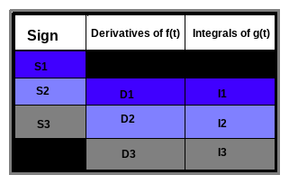
I’ve labeled the cells of this table to help you visualize the structure of the integral’s result. By overlaying this labeled table onto our original one, we can see that the indefinite integral should take the following form:

$\displaystyle \int t^{2}e^{-2}dt = (S_1)(D_1)(I_1) + (S_2)(D_2)(I_2) + (S_3)(D_3)(I_3)$

$\displaystyle = (+1)(2t)(-e^{-t}) + (-1)(2)(e^{-t}) + (+1)(0)(-e^{-t})$

$\displaystyle = -2te^{-t} - 2e^{-t}$

… therefore our definite integral becomes…

$\displaystyle \int \limits_{0}^{\infty} t^{2}e^{-2}dt = \lim \limits _{a \rightarrow \infty}[-2te^{-t} - 2e^{-t}]|_{t = 0}^{t = a} = 2$

which we know to be true, since

$\displaystyle \Gamma(3) = (3-1)! = 2$ .

We have just confirmed our near-trivial example, using tabular integration. Below is an excerpt that details how, when we explicitly consider the constants of integration, the terms containing them cancel out:

Demonstrating Elimination of Terms with Constants (click-here):

===================================

Using our example from before, we can reconstruct the first table:

Sign	Derivatives of $f(t)$	Integrals of $g(t)$
+	$t^{2}$	$e^{-t}$
–	$2t$	$- e^{-t} + C$
+	$2$	$e^{-t} + Ct + D$
–	$0$	$-e^{-t} +\frac{1}{2}Ct^{2} + Dt + E$

containing the constants $C$ , $D$ , and $E$ . Following the same pattern, our indefinite integral becomes:

$\displaystyle \int t^{2}e^{-2}dt = (S_1)(D_1)(I_1) + (S_2)(D_2)(I_2) + (S_3)(D_3)(I_3)$

$\displaystyle = (+1)(2t)(-e^{-t} + C) + (-1)(2)(e^{-t} +Ct + D)$

$\displaystyle + (+1)(0)(-e^{-t} + \frac{1}{2}Ct^{2} + Dt + E)$

… we can eliminate the last term here, as it contains a zero factor.

Further simplifying this expression:

$\displaystyle = -2te^{-t} + 2Ct - 2e^{-t} - 2Ct - 2D$

… the $2Ct$ terms cancel out, and we are left with…

$\displaystyle = -2te^{-t} - 2e^{-t} - 2D$ .

Now evaluating the definite integral, we observe that the term $-2D$ is eliminated:

$\displaystyle \int \limits_{0}^{\infty} t^{2}e^{-2}dt = \lim \limits _{a \rightarrow \infty}[-2te^{-t} - 2e^{-t} -2D]|_{t = 0}^{t = a} = 2$

==========================

Further Motivation

Interpolation of the factorial function via the Gamma function offers a broader perspective of interpolation altogether. Namely, I’ll pose the following question: given the mappings…

$\displaystyle q: \mathbb{Z} \longrightarrow \mathbb{Z}$

$\displaystyle q: \mathbb{Z} \longrightarrow \mathbb{R}$ ,

… satisfying preliminary assumptions required for interpolation, might integration serve as a general method? Proposing a family of integrable functions

$\displaystyle K(t, \mu)$

which I will call the interpolation kernel, the objective is to construct an interpolating function:

$\displaystyle Q(\mu) := \int \limits_{t_1}^{t_2} K(t, \mu) dt$

( $\displaystyle t_1, t_2 \in \mathbb{R}$ )

… such that $Q$ interpolates $q$ on some interval in $\mathbb{R}$ . Ideally if we let $K(t, \mu) = f(t)k(t, \mu)$ , this can be seen as a reframing of some integral transform:

$\displaystyle Qf(\mu) = \int \limits_{t_1}^{t_2} f(t)k(t, \mu) dt$

where $k$ is the kernel of our transformation, and $f$ is our function to be transformed. I hope it inspires you to look deeper into the Gamma function, and maybe explore this method of interpolation.

Here’s a relevant essay about the Gamma function by Philip J. Davis (click-here):

DavisGammaFunction Download

Share Your Feedback

BGecko

Learn how to see.

Developmental – Welcoming The Gamma Function

Leave a Reply Cancel reply

Share this:

Related

Leave a Reply Cancel reply