In Part I of our DSP Math Overview, we covered complex numbers and the closed-form solution for geometric series. Now, we will turn our attention to logarithms, their properties, and metric prefixes.

Logarithms

I’d like to begin part two of the math review with a section on logarithms and their properties. We will also cover some of the history of logarithms and their applications in DSP. Multiplying real numbers manually, and especially on early computational systems, can often be complex and tedious. Logarithms were originally developed to simplify calculations long before the computer was built. To explore this further, here’s an in-depth video on logarithms by Welch Labs:

As we can see, logarithms were originally developed in the 17th century as a powerful computational tool, particularly for simplifying complex calculations in navigation. This video illustrated how their fundamental utility lies in transforming multiplication into addition, a property given by the logarithmic identity:

for

Further mathematical exploration revealed that logarithms are the inverse of general exponential functions. More precisely, given the exponential relation:

we define the logarithm base , denoted by , as the function which retrieves the exponent:

Therefore the logarithm answers the question: to what power must be raised to yield ?. Here are a few examples of logarithmic functions :

#importing libraries

import numpy as np
import matplotlib
import matplotlib.pyplot as plt
matplotlib.style.use('ggplot')

# Generating plots

n = 3 # Number of plots
k = 5 # Scaling for b
N = [k*i for i in range(1, n+1)]
x = np.linspace(0, 15, 100)

for i in N:
  y = np.log(x)/np.log(i)
  plt.plot(x, y, '--')

plt.axhline(y=0,  color='gray') # designing the y axis
plt.axvline(x=0, color='gray') # designing the x axis

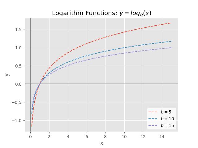
plt.title("Logarithm Functions: $y = log_b(x)$")
plt.xlabel("x")
plt.ylabel("y")
legend = plt.legend([f"$b = {s}$" for s in N])
legend.get_frame().set_facecolor('white')
plt.savefig("logarithms.jpg")

Observe in the graph that for any chosen base , we have . This follows from the fundamental identity , which holds for all . Furthermore, since for any , it follows that is undefined.

By convention, unless explicitly stated otherwise, the notation refers to the common logarithm, meaning the base is implicitly . Similarly, the natural logarithm is denoted by , where the base is Euler’s number .

Several key properties of logarithms follow from their definition:

Change of Base Formula:

Product Rule:

Power Rule:

These properties are essential in simplifying logarithmic expressions and solving exponential equations. Combining the Power and Product rules together, we have another rule:

Division Rule:

Metric Prefixes

Now lets investigate scaling. Surely you heard of the statement: “King Henry Died by Drinking Chocolate Milk,” which is commonly used for interpreting orders of magnitude. This mnemonic device corresponds to the metric prefixes:

“King”	“Henry”	“Died”	“by”	“drinking”	“chocolate”	“milk”
Kilo –	Hecto –	Deca –	base	deci –	centi –	milli –
k	h	D	—	d	c	m

Physical measurements, which quantify various properties and are expressed in units, can be conveniently modified with prefixes to indicate orders of magnitude. For instance, rather than stating that a signal has a frequency of one thousand Hertz (Hz), one can simply say it operates at one kilohertz (kHz).

Building upon this principle, I have developed an extended mnemonic system. Allow me to introduce The Great Monkey King:

Clearly, this regal primate has a taste for pancakes… perhaps as much as he enjoys “borrowing” unattended luggage at the airports. Thus, The Great Monkey King corresponds to the following table:

“The”	“Great”	“Monkey”	“King”
Tera –	Giga –	Mega –	Kilo –
T	G	M	K

From left to right, they scale down by 3 orders of magnitude for each prefix. Altogether, so far we have…

“The Great Monkey King Henry Dreamt by drinking cold milk.”

Notice the shift from “Died” to “Dreamt”, and from “chocolate” to “cold”. While some might speculate whether Henry met his end while sipping this not so chocolatey libation, the evidence clearly suggests he merely drifted into slumber in his cradle of bamboo and wicker…

It seems like he dozed off through the morning, so in the end, he made no pancakes…

“milk.”	“Made”	“no”	“pancakes.”
milli –	micro –	nano –	pico –
m		n	p

This is our final metric prefix table, summarizing the prefixes that, from left to right, decrease by three orders of magnitude. To help remember them, we have altogether:

“The Great Monkey King Henry Dreamt by drinking cold milk. Made no pancakes.”

If this mnemonic doesn’t resonate with you, try coming up with your own! Mnemonics are a great way to reinforce what we learn, and different people find different devices more effective. If you have a creative one, feel free to share it in the comments!