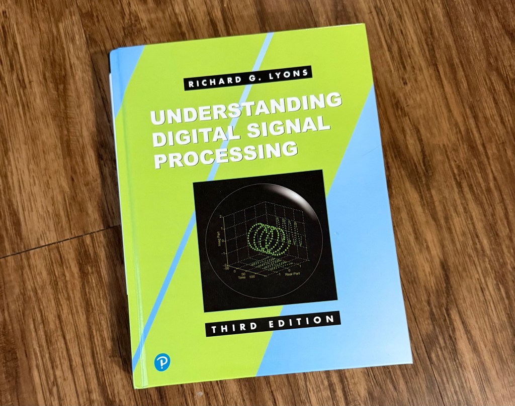
Foundational – DSP Notes: Math Overview (Part I)

Every image you see, every song you stream, every signal being transmitted across space… at its core, it’s all just numbers. Digital Signal Processing (DSP) is a silent architect of modern technology, with widespread Industrial and Scientific applications. This series was inspired by a conversation I had with my brilliant friend Rose, motivating us to explore the fundamentals of DSP this year. As yet, there’s no better guide than the Understanding Digital Signal Processing (UDSP) book by Richard Lyons, which we will undertake, starting with its mathematical foundations. However, these notes are not meant to be all-encompassing; rather, they serve as a supplement to Lyons’s book.

Complex Numbers

On Noteworthy Forms of Complex Numbers
and their Relationship

Appendix A of UDSP briefly summarizes complex numbers and their key properties. For a freshly intuitive grasp of these fundamentals, this video offers an excellent visual and conceptual framework:

Now assuming some familiarity with complex numbers, we will interpret their Trigonometric and Exponential representations:

(Trigonometric Form)

$\displaystyle z = M [\cos{\theta} + j \sin{\theta}]$

(Exponential Form)

$\displaystyle z = M e^{j \theta}$

The standard (rectangular) form of a complex number is $z = R+j I$ , with its conjugate $z^{*} = R-j I$ . The rectangular form emphasizes the real and imaginary components, while the two alternative forms highlight the magnitude and phase, offering insights into the vector’s length and direction in the complex plane. For any complex number $z$ in rectangular form, the magnitude and phase can respectively be determined as follows:

$\displaystyle M = \sqrt{R^{2} + I^{2}}$

$\displaystyle \theta = \tan{^{-1}\frac{I}{R}}$

But how can we show that the Trigonometric and Exponential forms represent the same concept? Since both forms share the same magnitude $M$ , demonstrating their equivalence reduces to proving:

$\displaystyle e^{j \theta} = \cos{\theta} + j \sin{\theta}$

To demonstrate this, we revisit pertinent concepts from differential calculus. Recall the Taylor series: for any infinitely differentiable function $f(x)$ , it can be expressed as an infinite sum:

$\displaystyle f(x) = \sum_{n = 0}^{\infty} \frac{f^{n}(a) (x - a)^{n}}{n!}$

where

$\displaystyle f^{n}(x) = \frac{d^{n}f}{dx^{n}}$ and $a \in \mathbb{C}$

When $a = 0$ , this series is referred to as the Maclaurin series. The following Maclaurin series expansions are instrumental in our derivation:

$f(x)$
$\sin{x}$	$= x - \frac{x^3}{3!} + \frac{x^5}{5!} - \frac{x^7}{7!}+ ...$
$\cos{x}$	$= 1 - \frac{x^2}{2!} + \frac{x^4}{4!} - \frac{x^6}{6!} + ...$
$e^{x}$	$= 1 + x + \frac{x^2}{2!} + \frac{x^3}{3!}+...$

To demonstrate $e^{j\theta} = \cos{\theta} + j \sin{\theta}$ , substitute $x = j \theta$ into the Maclaurin series for $e^{x}$ :

$\displaystyle e^{j \theta} = 1 + j \theta - \frac{\theta^2}{2!} - j \frac{\theta^3}{3!} + \frac{\theta^4}{4!} + j \frac{\theta^5}{5!}..$

… now we’ll group the real and imaginary terms…

$\displaystyle = (1 - \frac{\theta^2}{2!} + \frac{\theta^4}{4!} - \frac{\theta^6}{6!} + ...) + j (\theta - \frac{\theta^3}{3!} + \frac{\theta^5}{5!} - \frac{\theta^7}{7!} + ... )$

$\displaystyle = \cos{\theta} + j \sin{\theta}$

This fundamental result, called Euler’s formula, beautifully ties together exponential and trigonometric functions, forming the cornerstone of complex analysis and DSP.

On Conjugacy

In the context of complex numbers, the conjugate of a number reflects it across the real axis in the complex plane. Recall that $\sin{x}$ is an odd function, satisfying $\sin{-x} = - \sin{x}$ , and $\cos{x}$ is an even function, satisfying $\cos{-x} = \cos{x}$ . This is relevant, because we can use it to show the conjugate of the exponential form.

Given

$\displaystyle z = M e^{j \theta} = M [\cos{\theta} + j \sin{\theta}]$ ,

the conjugate can be expressed by

$\displaystyle z^{*} = M [\cos{\theta} - j \sin{\theta}]$

$= \displaystyle M [\cos{- \theta} + j \sin{- \theta}]$

$\displaystyle = M e^{- j \theta}$

The exponential representation of complex numbers is widely preferred, succinctly conveying both magnitude and phase. Notably, in any exponential expression $e^{x}$ , the exponent $x$ must be dimensionless to maintain mathematical consistency.

Use Radians!

While degrees are a common unit for measuring angles, they are not dimensionless. In contrast, radians are dimensionless quantities, making them the preferred unit in mathematical expressions involving exponents. To briefly explain it in order to gain more intuition, I’ll introduce the formula for arc length

$\displaystyle S = r \theta$

which can be rearranged to

$\displaystyle \theta = \frac{S}{r}$

… and we can see our angle $\theta$ is equal to one radian when $S = r$ , as depicted in the image below.

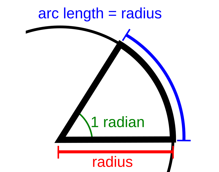
Image describing one Radian
(pulled from Wikipedia)

This is how we conceptualize one radian measure!

Complex Numbers Describe Rotations in the Complex Plane

In modern physics and engineering literature, complex numbers are often expressed in their exponential form for compactness and clarity. In DSP, where signals are time-dependent, the exponent is frequently written as $j \omega t$ , where $t$ represents time (in seconds) and $\omega$ denotes angular frequency, measured in radians per second.

$\displaystyle z(t) = M e^{j \omega t} = M e^{j \Theta(t)}$

where

$\displaystyle \frac{d \Theta}{dt} = \omega$

The UDSP book does not explicitly define the phase angle, $\Theta = \Theta(t)$ , in the appendix. However, in more advanced or physically realistic scenarios, $\Theta$ evolves as a function of time. For now, we will assume $\Theta = \omega t$ as given.

Lyons states that “the expression $z = M e^{-j \omega t}$ represents a phasor … that rotates in a clockwise direction about the origin of the complex plane at a negative radian frequency of $- \omega$ radians per second.”

To make sense of this, here is a brief video posted by u/westbeach013 on reddit, depicting the counter-clockwise rotations of $M e^{j \omega t}$ :

Exploring the beauty of Euler’s Formula in 3D! 🌀✨️
byu/westbeach013 inmathematics

Geometric Series

Lyons introduced the closed-form expression of a geometric series and provided a brief explanation. However, let’s explore it further and analyze it in more detail. We were given the following closed-form expression:

$\displaystyle \sum\limits_{n = p}^{N-1} r^{n} = \frac{r^{p} - r^{N}}{1-r}$

… but why is it relevant? Well, this closed-form expression allows us to compute the sum of our geometric series, without needing to calculate each term individually. Before proving the closed form, I’d like to introduce a compact notation that is relevant for proving theorems about geometric series. Define $X$ and $X_{N}$ as follows:

$\displaystyle X = 1 + r + r^{2} + r^{3} + ...$

and

$\displaystyle X_{N} = 1 + r + r^{2} + r^{3} + ... + r^{N}$

Convergence of X

I will leave as a task to the reader, to demonstrate that for any whole number $k$ :

$\displaystyle r^{k}X = X - X_{k-1}$

and

$\displaystyle r^{k}X_{N} = X_{N+k} - X_{k-1}$

Therefore $rX = X - 1$ , and so forth. Let’s first prove the statement:

$\displaystyle X = \frac{1}{1-r}$

for any $|r| < 1$ . We can confirm, by the distributive property, that

$\displaystyle (1-r) X = X - rX$

$\displaystyle = X - (X - 1)$

$\displaystyle = 1$

Therefore, since $(1-r) X = 1$ , we can be sure that, by elimination,

$\displaystyle X = \frac{1}{1-r}$ ,

provided that $|r| < 1$ . Now you might be wondering why this inequality constraint is necessary. Using the distributive property from algebra, we can demonstrate:

$\displaystyle (1-r) X_{N-1} = X_{N-1} - rX_{N-1}$

$\displaystyle = X_{N-1} - (X_{N} - 1)$

$\displaystyle = 1 - r^{N}$

So, then another equation worth remembering would be the following:

$\displaystyle X_{N-1} = \frac{1 - r^{N}}{1 - r}$

Now we can observe the limit of this equation as $N$ approaches infinity.

$\displaystyle X = \lim\limits_{N \to \infty} X_{N-1} = \lim\limits_{N \to \infty} \frac{1 - r^{N}}{1-r}$

When $|r| < 1$ , the $r^{N}$ quickly reduces to zero, yielding $\frac{1}{1-r}$ as a result. However, when $|r| > 1$ , our infinite sum $X$ explodes (i.e. it becomes divergent).

Proving the Closed-Form

Returning to the closed form expression, we can derive a simplified representation through a straightforward proof. Beginning with he summation, we arrive at its simplified form:

$\displaystyle \sum\limits_{n=p}^{N-1}r^{n} = X^{N-1} - X^{p-1}$

$\displaystyle = - \{X^{p-1} - X^{N-1}\}$

$\displaystyle = - \{\frac{1-r^{p}}{1-r} - \frac{1-r^{N}}{1-r}\}$

$\displaystyle = \frac{r^{p} - r^{N}}{1-r}$

Up to this point, we have explored complex numbers and their properties, the significance of radians, and the closed-form expression for geometric series. In the next discussion, we will delve into logarithms and metric prefixes — along with other foundational concepts essential to digital signal processing.

BGecko

Learn how to see.

Foundational – DSP Notes: Math Overview (Part I)

2 thoughts on “Foundational – DSP Notes: Math Overview (Part I)”

Leave a Reply Cancel reply

Share this:

Related

2 thoughts on “Foundational – DSP Notes: Math Overview (Part I)”

Leave a Reply Cancel reply