So what about those pesky definite integrals? I mean the ones integrating over a high number of dimensions. Many ML problems, especially in Bayesian statistics, involve computing probabilities or expectations over high-dimensional spaces. For this reason, we’re gonna need a clever way to compute these integrals.

Enter Monte Carlo Integration! This technique isn’t just a workaround; it’s a powerful tool that harnesses the power of randomness to estimate these integrals with surprising efficiency and accuracy. Imagine trading a laborious, exhaustive search for a clever, strategic sampling that yields equally valuable insights — that’s Monte Carlo Integration for you.

Monte Carlo Integration

Monte Carlo Integration’s elegance lies in its stochastic approach, diverging from deterministic methods like the Riemann sums approach and Trapezoidal rule. In contrast to strategically chosen points, Monte Carlo samples from a uniform distribution across the integration domain. Each random sample contributes to an integral estimate, relying on the principle that the average function value at these points are used to approximate the integral. The law of large numbers asserts that with large samples, our approximations progressively converge towards the true integral value.

In your calculus courses, you likely encountered the concept of determining the average value of a function over the interval . This is characterized by the following calculation:

Subsequently, we can articulate the integral across the domain through the following expression:

At first glance, this might seem challenging to calculate analytically. However, we can cleverly use randomness to our advantage here. By selecting random points from the continuous uniform distribution over , we can approximate . We do this through the formula

which is the average of the function values at these randomly selected points. To put this into a more tangible perspective, consider this: as the number of points increases indefinitely, our approximation gradually converges to the true average value . In mathematical terms, this is represented as

Now, when we multiply both sides of this equation by the interval length , it evolves into

This final equation is the central point of Monte Carlo Integration. It shows how, through the process of increasing , the approximation we get becomes an accurate representation of our original integral .

Monte Carlo Integration With Python

Lets dive into a straightforward yet illustrative example using python. This exercise will demonstrate the power of Monte Carlo Integration in action. To get started, ensure you have the necessary Python libraries installed. These libraries not only simplify our coding process, but also provide powerful tools to execute it efficiently.

# Importing Libraries
import numpy as np
import matplotlib
import matplotlib.pyplot as plt

Now, let’s define the function we intend to integrate. For our example, we’ll focus on a straightforward function:

In Python, we can briefly represent this function using lambda expression. Here’s how we implement our function in Python:

# Creating our function to integrate
f = lambda x: x**2  

We’ve selected this function for a specific reason: It’s simple enough to be calculated analytically, which allows us to validate our results. Let’s first compute the integral analytically over the domain for comparison purposes:

With the analytical solution in mind, we can establish a reference value in our Python code. This will allow us to later compare the outputs of the Monte Carlo method with this exact value, ensuring the accuracy of our stochastic approach.

Creating a python variable for

# Value of F(2, 3)
integral = 19/3.0

Let’s now move on to the computational side of Monte Carlo Integration. We define . As we’ve described earlier, theoretically,

This limit tells us that as the number of samples increases, our Monte Carlo estimate will get closer to the actual integral value. To simulate this in Python, we need a function for . This demands randomly sampling points from a uniform distribution over the interval and then computing the average value of at these points. Here’s how we can code this function in Python:

Creating

# Creating F^{k}(a,b)
def F(a, b, f, k):
  x = np.random.uniform(a, b, k)
  f_avg = (f(x).sum())/ float(k)
  return (b-a)* f_avg

Now lets put this integration function to the test. We aim to observe how the approximation of the integral improves as we increase the number of samples. To do this, we’ll compute the estimates for a range of values, starting from and going up to in increments of . This will give us a clear picture of how the accuracy of our method evolves with increasing sample sizes.

# Creating a list of domain values (k)
domain_k = [i for i in range(100, 100000, 10)]

# Creating a list of F^{k}(2, 3) values
approx_integ = [F(2, 3, f, i) for i in domain_k]

The list approx_integ stores the integral estimates for each in our specified range, and the domain_k list simply tracks the number of calculations performed, providing a handy reference for plotting or analyzing the results.

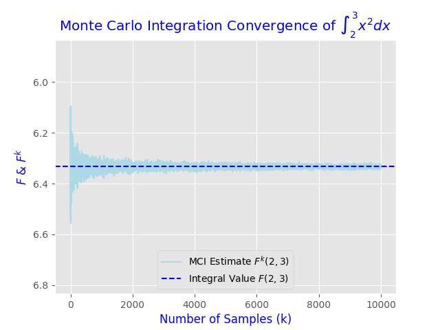
Finally, we can plot the values we obtained. We will use matplotlib, a popular Python library, for this purpose. The following code snippet sets up our plot with an appropriate style, legends, axis labels, and title, ensuring our visualization is informative and aesthetically pleasing.

plt.figure()
matplotlib.style.use('ggplot')

# Setting the bounds of the y-axis on our plot
plt.ylim(integral+.5, integral - .5)

# Creating plots
plt.plot(domain_k, approx_integ, color = "lightblue")  # Plotting F^{k}(2, 3)
plt.axhline(integral, color = 'blue', linestyle = '--' )  # Plotting F(2, 3)

# Legends, title, and labels
plt.legend(["MCI Estimate $F^{k}(2, 3)$", f"Integral Value $F(2, 3)$"], loc = "lower center")
plt.title("Monte Carlo Integration Convergence of $\int_{2}^{3} x^{2}dx$", color = 'blue')
plt.xlabel("Number of Samples (k)", color = 'blue')
plt.ylabel("$F$ & $F^{k}$", color = 'blue')

# Saving the figure (optional)
plt.savefig("mci_convergence.jpg")

In this plot, the blue dashed line represents the analytically calculated integral value of , while the light blue line shows the estimates obtained from Monte Carlo Integration for different values of . As increases, we expect the light blue line to approach and align more closely with the blue.

However the true elegance of this method is how it beautifully translates into integration over any number of dimensions. Unlike other traditional numerical integration methods, which often become increasingly complex and computationally intensive with each added dimension, Monte Carlo Integration maintains a consistent approach regardless of the number of dimensions involved.

Multiple Dimensions

Consider the task of computing the integral represented as

where is the integral of the function over the multi-dimensional domain . The procedure remains conceptually similar to the one-dimensional case, uniformly sampling points within , denoted as .

Our next step is to calculate the average value of the function over these points. The average, denoted as , is given by the formula:

It’s important to note that in the sum, each represents the function evaluated at the sampled point in the multi-dimensional space. As we increase the number of points ( ), according to the law of large numbers, this average value converges to the expected value of the function over the domain . In mathematical terms, this is represented as:

Here, represents the volume of our domain of integration. This volume, when multiplied by the average value of the function over the domain, gives us the approximate value of the integral , thus providing an effective method to calculate multi-dimensional integrals.

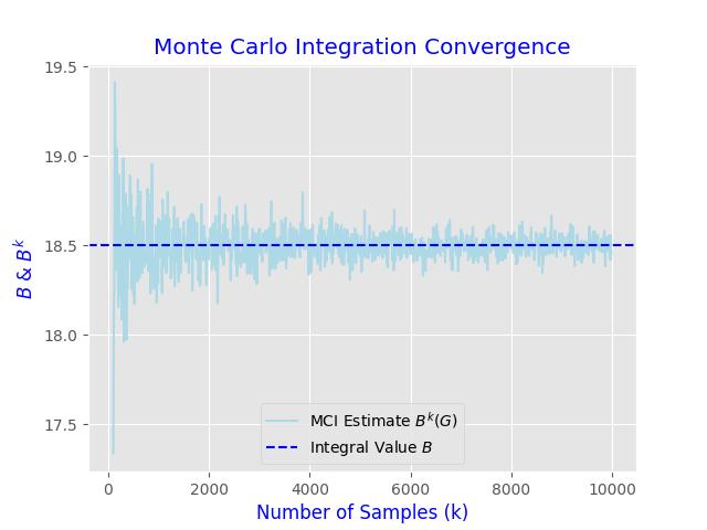
Lets illustrate this with a specific example. Imagine we want to calculate the integral of a function with two variables, x and y:

This integral represents the sum of the function over the rectangular region: . Analytically, computing this integral gives us a value of . This will allow us to gauge the accuracy of our Monte Carlo estimates.

The Python code provided below is designed to be versatile, capable of estimating integrals over spaces having dimensions greater than one. All it requires is the specification of the integration domain, the number of samples, and a function defined using Python’s lambda notation.

Compute

def compute_volume(G):
  vol = 1;
  for edge in G:
    vol *= (edge[1] - edge[0])
  return vol

Sample

def sample_domain(G, k_samples):
  d = len(G)
  edge_one = G[0]
  component_samples = np.random.uniform(edge_one[0], edge_one[1], k_samples)
  for edge in range(1, d):
    new_edge = G[edge]
    samples = np.random.uniform(new_edge[0], new_edge[1], k_samples)
    component_samples = np.vstack((component_samples, samples))
  return component_samples.T

Compute

def compute_integral(f, G, k_samples):
  volume = compute_volume(G)
  sample_points = sample_domain(G, k_samples)
  f_values = []
  for point in sample_points:
    f_values.append(f(*point))
  return volume * np.mean(f_values)

By sequentially running the code for various sample sizes, we can confirm these estimates converge towards the analytical value of 18.5:

Monte Carlo Integration is a reminder of how randomness and probability can be harnessed to uncover precise answers to intricate questions. As computational capabilities advance, the potential applications of this method are bound only by our imaginations. So lets immerse ourselves, explore creatively, and allow chance to lead us towards a fresh understanding and innovative answers.