What defines structure within a system, and how is it intertwined with the universe’s inherent randomness? This question is rooted in Erwin Schrödinger’s seminal work, “What is Life?”, where he introduces the concept of ‘negative entropy’ as a measure of a system’s structural integrity. For our analysis, let’s denote this as .

The intriguing aspect is its intrinsic connection to entropy of a system, traditionally understood to be a measure of disorder. We’ll represent this as (actual entropy). This leads to a compelling hypothesis:

In this equation symbolizes the maximum attainable entropy of a system . The essence of this relationship lies in its interpretative power. Consider the scenario where . This indicates an absence of structure within the system, leading to the conclusion that is in a state of complete disorder, i.e. .

In information theory, negentropy is typically defined through differential entropy, i.e. entropy of continuous distributions, comparing a given distribution to a Gaussian baseline to measure order. In this case, for some random variable with probability density function , the negentropy is given by:

where is the differential entropy of , and is the differential entropy of a Gaussian distribution with the same mean and variance as . While the Gaussian is known to have the maximum differential entropy, our formulation, embraces a broader more versatile spectrum. For sake of our analysis, lets rearrange this equation:

where we can view as being the “potential entropy” in a system. This relationship offers a window into understanding the balance between order & disorder in natural systems. It also invites us to contemplate the broader implications of this balance in fields ranging from physics to information theory. Drawing an analogy with the Hamiltonian formalism in physics is insightful here. Much like the Hamiltonian formalism, which provides a powerful approach to analyzing the dynamics of systems in physics, the concept of negentropy, as we have framed it, offers a similarly robust framework for examining various systems. In Hamiltonian mechanics, typically we employ the equation:

where and are respectively the kinetic and potential energy of a system. This framework is renowned for its versatility in handling a wide range of physical problems, and simplifies complex dynamics into a more manageable form. Similarly, this approach to negentropy proposes a more nuanced view of entropy that quantifies structure in a system.

Considering the temporal evolution of these variables reveals a fascinating aspect. We express it as follows:

This equation offers a window into the evolving nature of structure in a system. Particularly intriguing is the scenario where , indicative of a system that is both closed and isolated. In such a system, the rate of change of the negative entropy is represented as:

What does this imply? It suggests a profound conceptual truth: In a closed and isolated system, any increase in entropy is mirrored by a corresponding decrease in structure. In many AI/ML models, especially in controlled learning environments or simulations, systems are treated as closed and isolated for simplicity. Moreover, the negentropy is maintained constant over time to study specific behaviors in the system.

To illustrate these concepts, consider a coin flip as a concrete example, a simple system modeled by a Bernoulli distribution. Assume the probability of getting heads is , and the opposite outcome has probability . The entropy of this coin flip, again denoted as ​, measures the uncertainty or disorder of this outcome and is calculated as:

The maximum entropy of a coin flip scenario corresponds to an unbiased coin, where . The maximum entropy for such a fair coin flip is:

Now, integrating our concept of negentropy, , we can quantify it for our coin flip system as the difference between this maximum entropy and the actual entropy:

We can view the plot of entropy and negentropy as a function of p below:

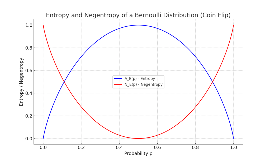
This plot presents negentropy in a manner that has inverse characteristics typically shown in standard entropy plots.

Until now, our exploration has paralleled the Hamiltonian perspective, emphasizing the total entropy as akin to a system’s total energy. Intriguingly, this invites us to consider an analogous form reminiscent of the Lagrangian approach in physics:

This formulation proposes a new way to view the interplay of entropy and negentropy, potentially offering a different angle to understand the dynamics of informational systems.

Extending Schrödinger’s insights into information theory and applying them to practical examples like a simple coin flip, deepens our appreciation of the dynamic interplay between structure and randomness. These frameworks also invite us to ponder the broader implications of these concepts in deciphering the complexity of the world around us.