Linear regression serves as a fundamental stepping stone into the world of machine learning, embodying both simplicity and the power of predictive analytics. Conceptually, it rests on a graceful mathematical framework that elegantly unravels its potential and delineates its limitations. This guide will walk you through the mathematical fundamentals, offering a clear exposition of its foundational principles. We will also assess how we can confront and circumvent these limitations, paving the way for more sophisticated analytical endeavors.

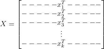
Envision a set of data points, each holding a story which can be better understood through the lens of linear regression. For , consider each data point as a vector within a d-dimensional space, , where each dimension corresponds to a different feature or measurement. Imagine the features of as coordinates plotted on a graph; each one marks a unique position on the axes, sketching the narrative of your dataset in a geometrical tableau.

Then we may compile these data points into a k-by-d data matrix, akin to a spreadsheet where each row is a data point and every column a distinct feature.

Corresponding to each data point in our matrix, there is an outcome or response, represented as a component of in the vector space .

Linear regression rests upon four critical assumptions that shape our analysis:

Assumption One: Linearity

The relationship between the independent variables and the dependent variable is linear, implying that it can be graphically represented by a straight line—or a hyperplane when —within the context of the model.

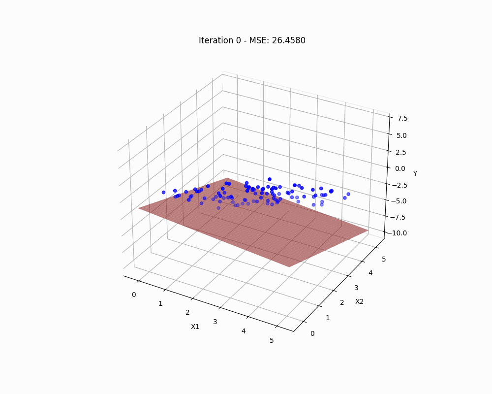
While the complexities of real-world phenomena often defy simple patterns, in the realm of linear regression, we distill these intricacies into a linear model that seeks the hyperplane most closely aligned with our data. We can describe this linear relationship using an equation that aims to determine the optimal “weights” or coefficients ( ) of our variables, while accounting for possible errors or noise in the data ( ):

In this equation, the term represents the feature vector ​ after being transposed and augmented with a 1 to incorporate the bias term as part of the weight vector . This bias term accounts for any offset from the origin in the model. The product of these vectors gives us the predicted value based on our model. Finally, represents the error term for the i-th data point, accounting for the deviation of the predicted value from the actual observed value . The goal in linear regression is to adjust the weights to minimize these errors across all data points.

If the equation above seems intricate, imagine it as finding the best-fit line through a scatterplot. By appending a column of ones to our matrix , we compactly model all observations with

,

where encapsulates the outcomes, and denotes our best-fit line, with accounting for any discrepancies.

Assumption Two: Homoscedasticity

The variability of the errors, which measure the vertical distances from our data points to the best-fit line, should remain constant across all levels of our independent variables. This concept, known as homoscedasticity, ensures that our model’s predictive accuracy doesn’t depend on the magnitude of the data points. Mathematically, we express this as the errors being normally distributed with a mean of zero and a constant variance, concisely written as .

Assumption Three: Independence of Observations

Independence of observations is key in linear regression; each data point must not be influenced by any other. This ensures that our model’s inferences are sound and unbiased. Mathematically, we express this as for , meaning the presence or position of one data point does not alter the likelihood of any other. This assumption is critical to avoid issues like autocorrelation–common in time series data–which can skew our model’s coefficients, compromising the model’s integrity, and undermining the validity of our predictions.

Assumption Four: Avoiding Multicollinearity

In linear regression, it’s essential that our independent variables, represented as ‘s, exhibit minimal correlation with one another. This phenomenon, termed multicollinearity, can obscure the individual effect of each variable, inflate the variance of the estimated coefficients, and compromise the interpretability of the model. Mathematically, we anticipate a correlation matrix of independent variables with off-diagonal elements close to zero, indicating low multicollinearity. We’ll delve into strategies to diagnose and rectify multicollinearity later, but for our initial model, we proceed under the assumption that such correlations are negligible.

Ordinary Least Squares Method

To identify the best-fitting line as described by our model, we need to find the weight vector that minimizes the discrepancy between the observed outcomes and the predictions . This discrepancy is encapsulated in the residuals , given by:

Our goal is to minimize the sum of the squares of these residuals, which is equivalent to minimizing their Euclidean norm squared:

Minimizing this quantity involves finding the weight vector that provides the smallest possible value for the squared residuals:

By expanding this expression, we aim to solve the optimization problem:

We can eliminate the first term here, since it is not a function of .

This formulation gives us the ordinary least squares solution (OLS) for the linear regression. The OLS method gives us the most efficient unbiased estimator under the Gauss-Markov theorem, assuming our previous four assumptions hold true.

To determine the optimal weights , we take advantage of the convex nature of our function. Convexity ensures that any local minimum is also a global minimum, and thus, the point where the gradient (or the first derivative with respect to ) of our function equals zero will give us the value of that minimizes the function. We calculate this by setting the derivative of our squared error term with respect to to zero:

Simplifying this expression by taking the derivative, we obtain:

By rearranging the terms, we get:

When is invertible, we can solve for the weight vector by multiplying both sides by the inverse of :

.

This solution is known as the Ordinary Least Squares (OLS) estimator. It gives us the set of weights that minimizes the squared residuals, thus providing the ‘best fit’ for our linear model under the least squares criterion. It’s important to note that this solution only exists when is invertible, which requires our data to be free of perfect multicollinearity, as discussed earlier.

An essential precondition for computing the matrix inverse is that the matrix has full column rank, meaning all columns (which represent our variables) are linearly independent. If this condition is not met, such as in the presence of multicollinearity, where variables are highly correlated, can become nearly singular. In practical terms, this can lead to large errors in the calculation of and unreliable regression estimates. Thus, confirming the absence of multicollinearity is not just a theoretical consideration but a computational necessity for the integrity of the OLS estimation.

Maximum Likelihood Estimation Approach

Building upon Assumption Two, we take a probabilistic approach to estimate using Maximum Likelihood Estimation (MLE). We start by recognizing that the residual is normally distributed as . This leads us to the probability density function (pdf) for :

With a substitution for , the pdf becomes:

Here, is posited as the “mean” of our predictions, with the observed outcomes distributed around this mean. To find the optimal , we turn to MLE, seeking the value of that maximizes :

Remarkably, this illustrates the equivalence between MLE under the assumption of normally distributed errors and the method of minimizing the sum of squared residuals, as we have previously shown with OLS. This equivalence bridges our statistical assumptions with practical estimation techniques. For a deeper dive into the MLE process, I invite the reader to reference my prior blog post on the topic.